 |
OpenStudioCore:analysis |
|
OpenStudioCore:analysis |
Base classes in alphabetical order:
All of the classes listed above, and the classes derived from them, derive from AnalysisObject, which follows the pImpl idiom, and specifies basic meta-data (UUID, version UUID, name, display name, and description). Because of the pImpl idiom, shallow copies of objects (made using assignment or copy construction) share data with each other. To get a deep copy, use AnalysisObject::clone.
Available analysis types:
The OpenStudio Analysis sub-project supports the formulation and solution of energy-efficient building design problems. Analysis works in concert with the entire analysis framework, see Figure 1.
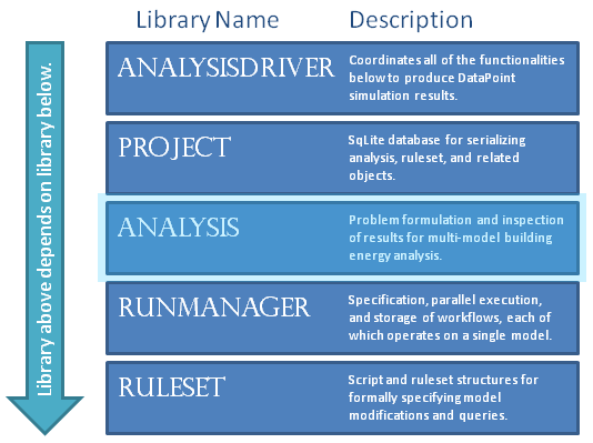
In particular, Analysis allows for the in-memory formulation of problems; problems are serialized to disk using project::ProjectDatabase and related classes; and problems are solved by instantiating Analyses with a seed model and running them using an analysisdriver::AnalysisDriver. AnalysisDrivers coordinate the operations of Analysis, Project, and RunManager, with the optional application of an Algorithm. Running an Analysis with an AnalysisDriver produces DataPoints, each of which provides an interface to the results of a single runmanager::Workflow (instantiated as a runmanager::Job with children).
To conduct an OpenStudio analysis, one must first formulate a Problem (or an OptimizationProblem, see Optimization). A Problem consists of a name, an ordered vector of WorkflowSteps, and an optional vector of response Functions. The WorkflowSteps, each of which represents an InputVariable or a runmanager::WorkItem, are maintained in a specific order to give users precise control over how a perturbed building model is created. For instance, if one variable adds Lights objects, and another variable changes the lighting power of all Lights objects, the order in which these variables are applied matters and should be explicitly set by the user. Analyses can be conducted on OSM, IDF, or a mixture of both; and in a debugging phase, one may not yet be interested in conducting simulations; thus we give the user precise control over all of the WorkflowSteps.
The Problem class was designed to be nominally shareable between projects, however, the practicality of sharing a given formulation will depend on the specifics of how the WorkflowSteps are defined.
A DiscreteVariable has a name, and consists of an ordered vector of DiscretePerturbations. Any InputVariable must implement InputVariable::createWorkItem, returning a runmanager::WorkItem that will set the variable to the appropriate value. For DiscreteVariables, this is equivalent to returning a WorkItem that will apply the DiscretePerturbation at the vector index passed to the createWorkItem method (as a QVariant of type Int). Therefore, the bulk of the createWorkItem work is performed by the individual DiscretePerturbation classes.
Each type of DiscretePertubation returns a different type of WorkItem. In particular, a NullPerturbation returns a null WorkItem that does nothing to its input model. A ModelRulesetPerturbation returns a WorkItem that will (when it is converted to a Job and run by RunManager) apply its ruleset::ModelRuleset to an OpenStudio Model, creating an output (perturbed) OpenStudio Model. A RubyPerturbation returns a WorkItem that will run a Ruby script on an input file, producing an output file. RubyPerturbations may run on OpenStudio models (OSM) or EnergyPlus models (IDF). What type of model is loaded as input, and what type is serialized as output, must be specified during the construction of a RubyPerturbation, either implicitly as part of a BCLMeasure, or explicitly using the FileReferenceType enumeration in utilities/core/FileReference.hpp.
ModelRulesetContinuousVariable works similarly to a DiscreteVariable with ModelRulesetPerturbations, except that it operates on a single (real-valued) attribute, and the value of that attribute is not specified up front. RubyContinuousVariables can be attached to individual ruleset::OSArguments in a Ruby script. Multiple such variables all referencing the same RubyPerturbation can be chained together as adjacent WorkflowSteps.
Individual runmanager::WorkItems can be placed anywhere in the Problem::workflow() vector. Almost always, some WorkItems for running EnergyPlus are placed toward the end of the workflow. For instance, if all of the InputVariables operate on OpenStudio Models, then the end of the workflow might be specified as:
You may also wish to specify a BCLMeasure with measureFunction() == MeasureFunction::Report as your final post-process step;
If any of your InputVariables operate directly on IDF, then you might want to create the InputVariable and then insert it before the EnergyPlusPreProcess job. Problem enables this with the method Problem::getWorkflowStepIndexByJobType, which inspects the runmanager::WorkItems in the Problem::workflow vector:
In addition to specifying how parametrically related models are to be generated, a Problem formulation may also specify the particular metrics that should be used to evaluate the resulting models. This is done with responses, which at this time must be LinearFunctions. Most of the time, at least one of the variables in a given response function will be of type OutputAttributeVariable.
OutputAttributeVariables call out an attributeName to be looked up after a DataPoint has been successfully simulated. The attributeName should correspond to an Attribute written out to a report.xml file produced by a post- processing job, see, for instance, runmanager::JobType::EnergyPlusPostProcess, and openstudio\runmanager\rubyscripts\PostProcess.rb (and similar scripts in that folder). The post-process job that produces the attribute called out by OutputAttributeVariable must be part of the Problem's workflow.
Once you have a problem formulation, you can construct an Analysis object by specifying a name, the Problem to be solved, and a seed model (OSM or IDF) in the form of a FileReference (utilities/core/FileReference.hpp). Whether or not you specify an Algorithm, you can always construct and add your own DataPoints to be run by an analysisdriver::AnalysisDriver.
To create a new DataPoint, a value for each of the Problem's variables must be specified using a std::vector<QVariant>. If the variable is discrete, the QVariant must be convertible to int, and as that integer will be interpreted as an index into DiscreteVariable::perturbations(false), it must be >= 0 and < DiscreteVariable::numPerturbations(false). If the variable is continuous, the QVariant must be convertible to double and should make sense in the context of that variable. In any case, the size of the std::vector<QVariant> must be equal to Analysis::problem().numVariables().
Once the variable values are specified, a new DataPoint is constructed by calling Problem::createDataPoint, and is added to the Analysis with Analysis::addDataPoint. Assuming the variable values were valid, and that a DataPoint with the same variable values is not already in the Analysis, the new DataPoint will now be in the list Analysis::dataPointsToQueue, and it will not have any results.
Algorithms are automated methods for generating DataPoints. OpenStudio contains two sorts of algorithms: OpenStudioAlgorithms, which are directly specified in the OpenStudio code base through the definition of OpenStudioAlgorithm::createNextIteration; and DakotaAlgoritms, which rely on DAKOTA (http://dakota.sandia.gov/software.html) to specify the variable values to run. Either type of algorithm may be specified during the construction of an Analysis. If present, the AnalysisDriver will call createNextIteration or kick off a runmanager::DakotaJob as appropriate.
If all of a Problem's variables are discrete, then a DesignOfExperiments Algorithm can be applied. If this is done, and the analysis is run with an analysisdriver::AnalysisDriver, DesignOfExperiments::createNextIteration will be called by the AnalysisDriver, and the resulting new DataPoints will be run, with the results serialized to a project::ProjectDatabase. At this time only full factorial analyses are supported, and all of the runs are queued in the first and only iteration of the algorithm.
If DAKOTA is installed on your system, then a ParameterStudyAlgorithm can be specified to do basic parameter scans. Types of scans that add to (rather than duplicate) what is available in OpenStudio without DAKOTA include ParameterStudyAlgorithmType::vector_parameter_study and ParameterStudyAlgorithmType::centered_parameter_study.
A DAKOTA DDACEAlgorithm can be specified to sample a parameter space stochastically (rather than deterministically like DesignOfExperiments and ParameterStudyAlgorithm). To get started, specify the sampling type in a DDACEAlgorithmOptions object using the enum DDACEAlgorithmType. By default, the DDACEAlgorithmOptions::seed will be explicitly set to support analysis restart (by AnalysisDriver in coordination with DAKOTA) in case of a runtime failure or disruption. See DDACEAlgorithmOptions and the DAKOTA documentation for detailed information.
FSUDaceAlgorithm is similar to DDACEAlgorithm, but provides different sampling methods, see FSUDaceAlgorithmType, FSUDaceAlgorithmOptions, and the DAKOTA documentation. By default, the FSUDaceAlgorithmOptions::seed will be explicitly set to support analysis restart (by AnalysisDriver in coordination with DAKOTA) in case of a runtime failure or disruption.
PSUADEDaceAlgorithm exposes the PSUADE Morris One-At-A-Time (MOAT) sensitivity analysis method available through DAKOTA, see PSUADEDaceAlgorithmOptions, and the DAKOTA documentation. By default, the PSUADEDaceAlgorithmOptions::seed will be explicitly set to support analysis restart (by AnalysisDriver in coordination with DAKOTA) in case of a runtime failure or disruption. See the DAKOTA documentation for detailed information.
The DAKOTA SamplingAlgorithm is like DDACE in that it provides random (Monte Carlo) sampling and latin hypercube sampling (LHS). In addition, it samples across a number of uncertainty description types, for both continuous and discrete variables. (DDACE only works with continuous variables. To make it more broadly useful, we sometime make our discrete variables look continuous to DAKOTA when using DDACE.) Such sampling enables sensitivity analysis and uncertainty quantification.
To use this algorithm effectively, create one or more UncertaintyDescriptions using GenericUncertaintyDescription or one of the UncertaintyDescriptionType-specific interfaces (e.g. NormalDistribution, LognormalDistribution, PoissonDistribution, HistogramPointDistribution).
As with the Dace algorithms, SamplingAlgorithm::seed is explicitly set by default, to support analysis restart (by AnalysisDriver in coordination with DAKOTA) in case of a runtime failure or disruption.
OpenStudio currently supports unconstrained optimization problems with two linear objective functions, and discrete variables.
An OptimizationProblem is a Problem that also has one or more objective functions. At this time, a LinearFunction class is provided for the purpose of constructing objective functions. Often, an objective will be a single high-level output variable as in:
Once a vector of Functions is created, along with all the information required for a basic Problem, an OptimizationProblem may be constructed and used in the same way. At this time, all objective functions are to be minimized, so if you want maximization, please multiply your objective function by -1 (by specifying appropriate LinearFunction coefficients).
OptimizationProblems with two objective functions and Problem::allVariablesAreDiscrete()), can be solved using the SequentialSearch algorithm.
SequentialSearch is a greedy heuristic algorithm that works by tracing out a "minimum curve" for one of the two objectives. Which objective is "minimized first" must be specified up front using the class SequentialSearchOptions. As the objective functions are indexed starting at zero, usually the index 1 would be specified, as this naturally corresponds to the y-axis on a plot of the objective function values. The minimum curve starts at the baseline point (first perturbation specified for each variable), and then moves always in the direction of improving the other objective function, that is, the objective function that is not minimized first. In previous work, an economic objective has been minimized first, while always improving an energy use objective, which works well here at NREL since we are not generally interested in cheaper buildings that use more energy. This methodology does not work as well when both objectives are equally important, such as when cooling energy and heating energy are traded off. However, this deficiency can be overcome by solving first with one, and then again with the other objective function being minimized first.